Why Does “Probability 0” Not Mean “Impossible”? | Probabilities of Probabilities, Part 2

TL;DR

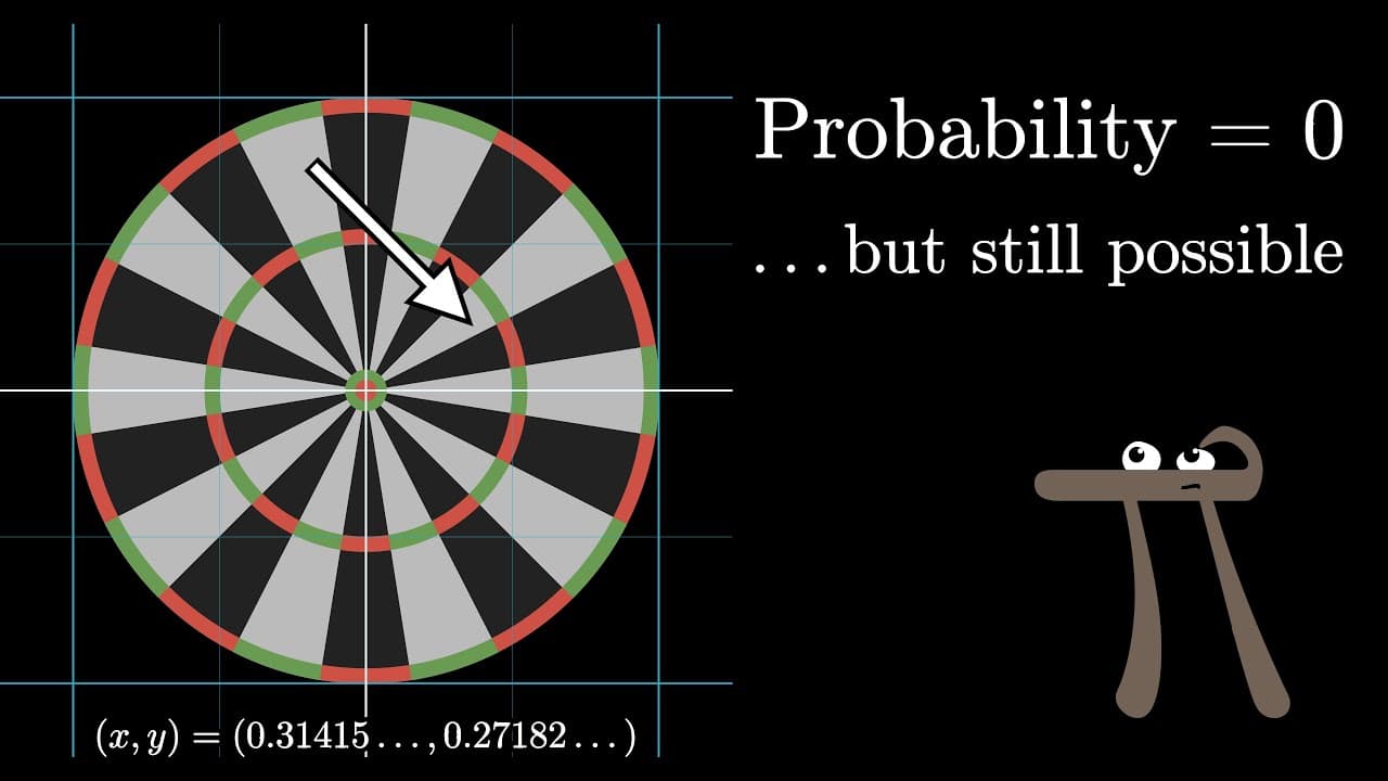
Probability zero does not mean impossible for an exact outcome in a continuous distribution because a single value occupies an infinitely thin slice with zero area. For an unknown coin weight h between 0 and 1, probabilities belong to ranges and equal areas under a probability density function, whose total area is 1. Read on to understand how density resolves the apparent paradox.

Transcript

Imagine you have a weighted coin, so the probability of flipping heads might not be 50-50 exactly. It could be 20%, or maybe 90%, or 0%, or 31.41592%. The point is that you just don't know. But imagine that you flip this coin 10 different times, and 7 of those times it comes up heads. Do you think that the underlying weight of this coin is such tha... Read More

Key Insights

• An unknown coin weight h is a real number from 0 to 1, representing outcomes from a coin that always lands tails to one that always lands heads, including every intermediate probability.
• Assigning positive probability to every exact value in a continuous range creates a problem because there are uncountably infinitely many possible values, while assigning zero to each appears to make their total zero instead of one.
• Ranges of values are the fundamental objects for continuous probabilities. Instead of asking only whether h equals precisely 0.7, a meaningful practical question asks whether h lies within an interval such as 0.6 to 0.8.
• Probability is represented by the area of each histogram bar, not its height. As buckets become narrower, their probabilities decrease through shrinking widths while their heights stay roughly stable, preserving and refining the distribution's overall shape.
• Probability density is probability per unit along the horizontal axis. Because a bar's probability equals width times height, its height expresses density, while areas over selected ranges express actual probabilities.
• A probability density function assigns density to individual inputs. The probability that a continuous random variable lies between two values equals the area under the density curve between those values, and the total area under the full curve equals one.
• An exact value in a continuous distribution has probability zero because it corresponds to an infinitely thin slice with zero area. All possible values together still have probability one because the full curve covers an area of one.
• Measure theory unifies discrete, continuous, and mixed probability settings. It can handle a random number that equals 0 with 50% probability while otherwise following a positive continuous distribution shaped like half of a bell curve.

Questions & Answers

Q: Why can a possible outcome have probability zero?

A possible exact outcome can have probability zero when values vary continuously. A single value is an infinitely thin slice with zero area under the probability density curve, while the area across the full range is 1.

Q: What is a probability density function?

A probability density function, or PDF, assigns probability density to the possible values of a continuous random variable. The probability of a value lying between two points equals the area under the curve between them, and the total area under the curve must equal 1.

Q: Why is the probability that the coin weight h equals exactly 0.7 zero?

The unknown heads probability h can be any real number from 0 to 1. The exact value 0.7 corresponds to an infinitely thin slice under the density curve, so its area, and therefore its probability, is 0.

Q: How should probabilities for an unknown weighted coin be expressed?

They should be expressed for ranges of possible coin weights rather than individual values. For example, one can ask for the probability that h lies between 0.8 and 0.85, with that probability represented by the area assigned to the interval.

Q: Why does area represent probability in a continuous distribution?

As histogram buckets become finer, their widths and individual probabilities approach zero while their heights remain roughly stable. Using width multiplied by height preserves the distribution’s overall shape and keeps the total area equal to 1.

Q: What does the height of a probability density curve represent?

The height represents probability per unit along the horizontal direction, which is called probability density. It is not the probability of an exact value; an interval’s probability comes from the area across its width.

Q: How do histogram buckets become a smooth probability density curve?

The ranges are divided into progressively finer and narrower buckets, with each bucket’s area representing its probability. Their probabilities shrink with their widths, but their heights remain roughly stable, so the histogram approaches a smooth curve without losing the distribution’s shape.

Q: How is the continuous probability paradox resolved?

The paradox is resolved by assigning probabilities to ranges and densities to individual inputs. Every exact value can have probability 0 while the full continuum has probability 1 because probability is measured by area rather than by adding the probabilities of uncountably many individual points.

Summary & Key Takeaways

• For a weighted coin with unknown heads probability h, asking for the probability that h equals exactly 0.7 creates an apparent paradox. Uncountably many individual values cannot all receive positive probabilities, yet assigning zero to each seems unable to produce the required total probability of one across every possible value.

• The paradox is resolved by treating ranges, rather than individual values, as the fundamental objects carrying probability. As increasingly narrow buckets approach a smooth curve, each bucket's probability shrinks with its width while its height approaches probability density. Probability is therefore represented by area, and the total area must equal one.

• A probability density function answers continuous probability questions through areas under its curve. An exact value has probability zero because its slice has zero width, while an interval can have positive probability. Measure theory provides a rigorous framework that unifies discrete, continuous, and mixed distributions under compatible rules for assigning probability to sets.