How Does the Central Limit Theorem Work?

TL;DR

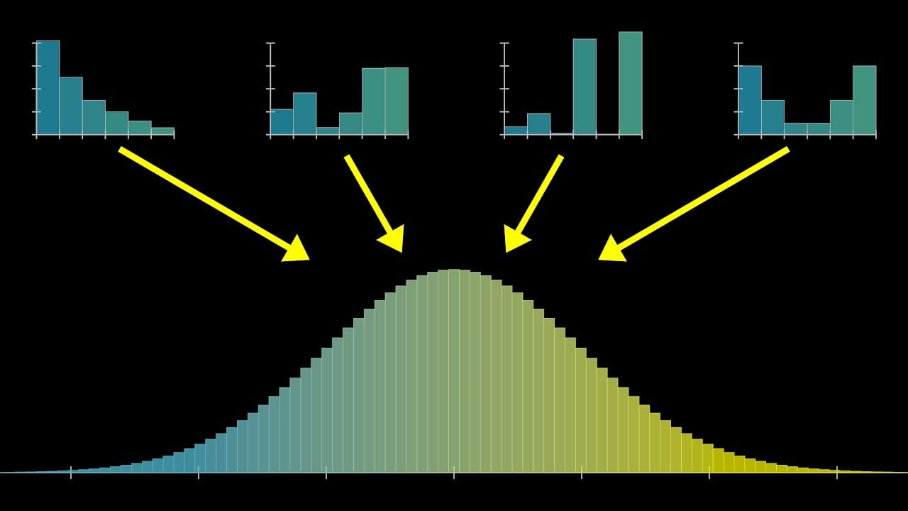
Adding more independent samples of the same random variable produces a sum whose distribution looks increasingly like a normal, or bell-shaped, curve. This pattern can emerge even when the original distribution is weighted, skewed, or concentrated near extreme values, allowing probabilities for large sums to be approximated and used to identify likely ranges.

Transcript

This is a Galton board. Maybe you've seen one before, it's a popular demonstration of how, even when a single event is chaotic and random, with an effectively unknowable outcome, it's still possible to make precise statements about a large number of events, namely how the relative proportions for many different outcomes are distributed. More speci... Read More

Key Insights

• A random variable is a random process whose possible outcomes are associated with numbers. A peg bounce can be represented by negative one or positive one, while a die roll is represented by one of its six numbered outcomes.
• The central limit theorem says that the distribution of a sum looks increasingly like a bell curve as the number of sampled random variables in that sum grows. The distribution describes how likely the sum is to take each possible value.
• A simplified Galton board represents a ball's final position as the sum of repeated 50-50 choices. Each bounce adds one or subtracts one, so five rows produce a sum formed from five random numbers.
• A normal distribution is also called a bell curve or a Gaussian distribution. It appears in seemingly unrelated settings, including the heights of people in a similar demographic and the numbers of distinct prime factors found in large natural numbers.
• A bell-shaped distribution can emerge from an asymmetric starting distribution. Simulations using a weighted die skewed toward lower values become more symmetric as the number of dice included in each sum rises from two toward larger sample sizes.
• The individual outcomes do not need to be equally probable in the dice examples. A bell-curve shape still emerges when most probability is concentrated on one and six, with very little probability assigned to the middle values.
• A simulation estimates a distribution by repeating the same sampling process many times and recording each sum. A finite run can look spiky because of randomness, so theoretical calculation is needed to reveal the precise long-run distribution.
• A uniform pair of dice turns the probability distribution of their sum into a counting problem. Every ordered pair has probability 1 in 36, so counting the pairs along each equal-sum diagonal gives the exact distribution for two dice.

Questions & Answers

Q: What does the central limit theorem say?

The central limit theorem says that when multiple samples of a random variable are added, the probability distribution of the resulting sum looks increasingly like a normal, or bell-shaped, curve as the size of the sum grows. The lesson presents this as the central idea, then develops it quantitatively so that the distribution can support predictions about large sums.

Q: How does a Galton board illustrate the central limit theorem?

In the simplified Galton board, a ball encounters a sequence of pegs and has a 50-50 chance of moving left or right at each one. Those movements are represented as negative one and positive one. The final bucket corresponds to their sum, while many balls show the relative frequency of each possible sum. Adding more rows makes the resulting distribution look more bell-shaped.

Q: What is a random variable in probability?

A random variable is shorthand for a random process in which every possible outcome is associated with a number. A bounce from a peg is modeled with two outcomes, negative one and positive one. Rolling a die provides another example, with six different outcomes associated with numbers. Multiple samples of such a variable can then be added and studied as a distribution.

Q: Why does a bell curve appear when adding dice rolls?

A bell curve appears because the distribution of a sum becomes increasingly bell-shaped as more samples of the same die-roll variable are included. In the simulations, adding only two dice leaves a shape resembling the original skewed distribution. Sums of five, ten, and fifteen dice become progressively more symmetric, with a central lump and probabilities that fade toward the tails.

Q: Does the central limit theorem require a fair die?

The dice demonstrations show that equal probabilities are not required for the central pattern being illustrated. A die can have a distribution skewed toward lower outcomes, yet repeated sums still become increasingly bell-shaped. The same effect appears when most probability is assigned to outcomes one and six and very little is assigned to the middle values. The theorem does, however, have three assumptions discussed later in the lesson.

Q: How can you calculate the distribution for two fair dice?

For two dice whose six faces each have probability one sixth, every possible ordered pair has the same probability, 1 in 36. Calculating the distribution is therefore a counting exercise. Group the pairs according to their shared sum, which can be visualized as diagonals in a grid, then count the number of pairs in each group to obtain the exact shape.

Q: Why are simulations alone insufficient for studying distributions?

Simulations provide a useful picture by repeating a sampling process many times and recording the resulting sums, but a finite run retains visible randomness. In the example stopped at 3,000 samples, the distribution looks broadly bell-shaped while its buckets remain spiky. That makes it unclear whether individual irregularities reflect the true distribution or merely random variation, motivating a theoretical calculation of the long-run shape.

Q: How can the central limit theorem help predict a large sum?

The theorem can be used to identify a range in which a large random sum is likely to fall. The lesson's concrete example asks for the smallest range that contains the total of 100 die rolls with 95% confidence. The approach applies whether the die is fair or weighted, once the distribution is described using the quantitative ideas developed in the lesson.

Summary & Key Takeaways

• A simplified Galton board models every bounce as a 50-50 choice between adding one and subtracting one. After five rows, the ball's final position is the sum of five random choices. Releasing many balls reveals how frequently the possible sums occur, producing a distribution across the board's buckets.

• The central limit theorem describes what happens when multiple samples of a random variable are added. As the number of terms in each sum increases, the resulting distribution looks increasingly like a bell curve. Dice simulations show this progression even when individual outcomes have unequal probabilities or a strongly asymmetric distribution.

• The theorem makes probability questions about large sums manageable. One example asks for the smallest range that has a 95% chance of containing the total from 100 die rolls. The lesson connects this application with normal distributions, mean, variance, standard deviation, sample means, the Gaussian formula, and three required assumptions.