How to Draw a Round Robin Gantt Chart With Arrival Times

TL;DR

Build the Gantt chart first, then compute averages. With a 2-unit time quantum, each running process is preempted when the quantum expires, and the CPU goes to the process at the head of the ready queue. A preempted process is always placed last, behind any process that arrived at that same instant, with its remaining burst time carried forward.

Transcript

in the previous lecture we have discuss about round-robin scheduling and we have also taken a small example and have seen how it works so in this lecture we will be solving another problem all around drop-in scheduling so let us see what is this problem so here it says consider the set of five processes whose arrival time and burst time are given b... Read More

Key Insights

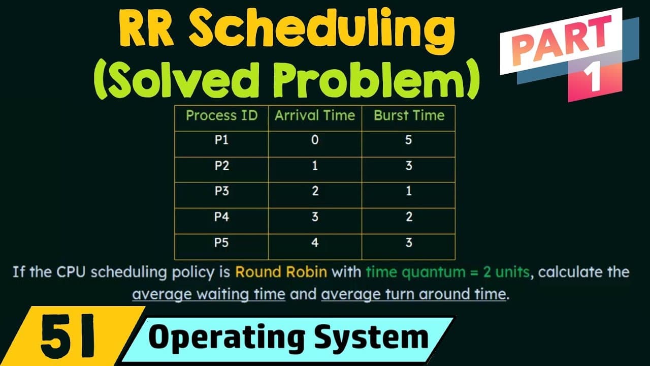
• The problem asks for average waiting time and average turnaround time for five processes P1 through P5 with given arrival times and burst times, under a round robin policy with a time quantum of 2 units.
• The difference from the previous lecture's example is that arrival times are now given, whereas earlier all processes were assumed to arrive at the same time, which made the calculation easier.
• Forming the Gantt chart is the most crucial step, which is why the lecture is split into two parts: part one builds the chart, and part two computes the average waiting time and average turnaround time.
• The ready queue holds processes waiting for the CPU, with the right hand side as the head and the left hand side as the tail; a process is removed from the ready queue the moment it receives the CPU.
• A preempted process is always placed last in the ready queue, behind any process that arrived at the same time unit, which is why P3 goes ahead of P1 at time 2 and P5 goes ahead of P2 at time 4.
• Remaining burst time must be tracked at every preemption: P1 has a burst time of 5 and runs 2 units, leaving 3 units; P2 has a burst time of 3 and runs 2 units, leaving 1 unit.
• A process whose remaining burst time is shorter than the time quantum releases the CPU voluntarily before the quantum ends, so no alarm rings; P3 has a burst time of only 1 unit and finishes at time 5.
• The ringing alarm in the walkthrough marks the end of a time quantum, signalling that the running process must be preempted and the CPU handed to the process at the head of the ready queue.

Questions & Answers

Q: How do you form a Gantt chart for round robin scheduling when arrival times are given?

Step through the timeline one unit at a time while maintaining a ready queue. At each instant, check the table for newly arrived processes and add them to the tail of the queue. When the time quantum expires, preempt the running process, place it at the very end of the queue behind anything that arrived at that same instant, and give the CPU to the process at the head of the queue. Record each CPU allocation as a block in the Gantt chart, and keep track of the remaining burst time of every preempted process.

Q: What is the time quantum used in this round robin problem?

The time quantum in this problem is 2 units. The CPU scheduling policy is round robin with a quantum of 2 units, meaning each process is allowed to execute for at most 2 units of time before it is preempted and the CPU is handed over to the next process waiting in the ready queue. The clock in the walkthrough rings an alarm every time 2 units of execution are complete, such as at time 2 and again at time 4, to signal that a preemption is due.

Q: Why is a preempted process placed at the end of the ready queue?

Round robin gives each waiting process a fair turn, so a process that has just used its full time quantum must go behind everyone else. The rule stated in the lecture is that the process that is preempted will always be the last one in the queue. This matters when another process arrives at exactly the same time unit as the preemption: at time 2, P3 arrives and P1 is preempted, so P3 is placed first and the preempted P1 goes behind it. The same happens at time 4 with P5 ahead of the preempted P2.

Q: What happens if a process finishes before its time quantum expires?

It voluntarily releases the CPU and the next process in the ready queue starts immediately, with no alarm ringing because the quantum was never reached. In this problem, P3 receives the CPU at time 4 but has a burst time of only 1 unit, which is less than the 2 unit quantum. So at time 5, P3 completes its execution, releases the CPU on its own, and the CPU passes to P1, which is at the head of the ready queue at that moment.

Q: How do you calculate the remaining burst time after a preemption?

Subtract the time already executed from the total burst time. P1 has a burst time of 5 units and executes from time 0 to time 2, which is 2 units, so 3 units remain and P1 is placed back in the ready queue with that remaining requirement. Similarly, P2 has a total burst time of 3 units and executes from time 2 to time 4, so 1 unit remains. Tracking these leftovers is essential because the process must return to the CPU later to finish.

Q: What is the difference between the head and the tail of the ready queue?

In the diagram used in this lecture, the right hand side of the ready queue represents the head and the left hand side represents the tail. The first process to arrive sits at the head, the second arrival is placed behind it, the third behind that, and so on. The process at the head is the one that gets the CPU next. Once a process receives the CPU, it is removed from the ready queue entirely, because the ready queue only holds processes that are waiting for the CPU.

Q: When does a process leave the ready queue in round robin scheduling?

A process is removed from the ready queue at the moment it is given the CPU. The ready queue holds only processes that are waiting for the CPU, so once a process begins executing it moves into the Gantt chart instead. This is shown at time 0, when P1 is taken out of the queue as it starts running, and again at time 2 when P2 is removed as it receives the CPU, and at time 4 when P3 is removed as it starts.

Q: Why is this round robin problem harder than the previous lecture's example?

In the previous lecture, arrival times were not given and it was assumed that all processes arrived at the same time, which made the calculation relatively easy. In this problem the arrival times are supplied for each of the five processes, so the arrivals must be tracked alongside the preemptions at every time unit. That means deciding, at each instant, which process joins the ready queue first when an arrival and a preemption coincide. The lecture stresses being very attentive and careful rather than the problem being conceptually difficult.

Summary & Key Takeaways

• The problem gives five processes, P1 to P5, each with an arrival time and a burst time, and asks for the average waiting time and average turnaround time under round robin scheduling with a time quantum of 2 units. Because arrival times are supplied, the solution requires more care than the earlier same-arrival example.

• The walkthrough uses a clock to step through each time unit alongside a Gantt chart and a ready queue. At time 0, P1 arrives and immediately gets the CPU. At time 1, P2 arrives but must wait because P1 has not exhausted its quantum. At time 2, the quantum expires and P1 is preempted with 3 units remaining.

• At time 2, P3 also arrives, so P3 enters the queue ahead of the preempted P1, and P2 starts running. P4 arrives at time 3. At time 4, P2 is preempted with 1 unit left, P5 arrives and is queued ahead of P2, and P3 begins. P3 needs only 1 unit, so it finishes at time 5 and voluntarily hands the CPU to P1.