How to Solve Linear Programs Graphically

TL;DR

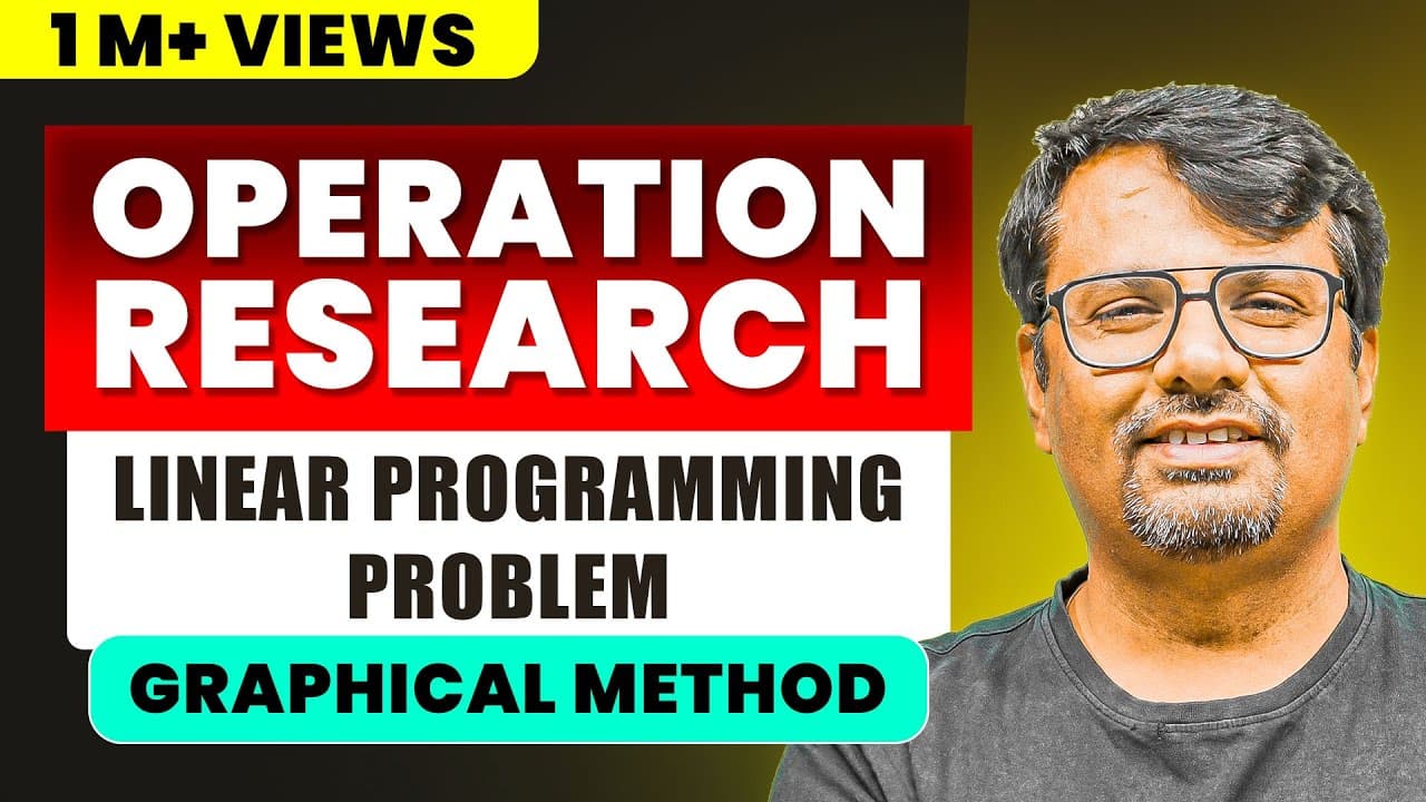
Graphical linear programming begins by identifying the common feasible region and then evaluating where the objective reaches its required result. The method also distinguishes unique optima from unbounded, infinite or alternate solutions, and cases with no solution. If two points produce the same optimal value, every point between them also produces that value.

Transcript

Hello students myself Dr. Gajendra Purohit and I have done my Phd in algebra and I have also cleared my CSIR-NET and my videos are for engineering mathematics and bsc students uploaded you all might face a lot of problem as many students ask that where are these videos so please if you are facing any problem then here is a playlist so you can go th... Read More

Key Insights

• The graphical method is a procedure for solving linear programming problems by examining their constraints, common feasible region, and objective results. The lecture develops the procedure through six questions intended for engineering mathematics, basic science, and several examination audiences.
• A feasible region is central to the graphical interpretation of a linear programming problem. The instructor treats it as one of the essential concepts needed to determine whether the constraints share an acceptable region in which a solution can be considered.
• An optimal solution is the objective result selected from the feasible possibilities. The lecture distinguishes this concept from degeneracy, unbounded solutions, infinite or alternate solutions, and no-solution cases so that different graphical outcomes are not incorrectly treated as equivalent.
• An unbounded solution occurs in the discussed cases when a solution exists but the required objective result does not have the necessary bound. The instructor explicitly notes that such problems still have solutions, even though their classification is unbounded.
• An infinite solution occurs when the objective does not have a unique optimal point. The lecture connects this outcome with alternate solutions and emphasizes that the repeated objective value must be recognized rather than reported as a single unique answer.
• Two points with the same objective value imply that every point between them also gives that same value. In the example described by the instructor, the shared value is 6, so the complete segment represents infinitely many solutions.
• A no-solution case occurs when the constraints do not produce a common feasible region from which an answer can be obtained. The graphical method therefore supports classification as well as calculation by revealing incompatible constraint conditions.
• The simplex method is presented as the next technique for solving these types of linear programming problems. The instructor states that a simplex table can also be used to identify an infinite-solution result, extending the graphical concepts into a tabular method.

Questions & Answers

Q: How do you solve a linear programming problem graphically?

A linear programming problem is solved graphically by representing its constraints, identifying their common feasible region, and determining the objective result within that region. The lecture uses six questions to demonstrate the method and stresses that the final interpretation must classify the outcome correctly as optimal, unbounded, infinite or alternate, or no solution.

Q: What is the feasible region in graphical linear programming?

The feasible region is the common region associated with the constraints of a graphical linear programming problem. According to the lecture, identifying this region is necessary before deciding what result the problem has. If no common feasible region is available from which an answer can be obtained, the problem is classified as having no solution.

Q: What is an optimal solution in linear programming?

An optimal solution is the selected objective result obtained from the feasible possibilities in a linear programming problem. The lecture treats optimality as distinct from degeneracy, unboundedness, infinite or alternate solutions, and no-solution outcomes. A result should not be called uniquely optimal when multiple points produce the same objective value along the region being examined.

Q: What does an unbounded solution mean in linear programming?

An unbounded solution describes a case in which solutions exist, but the required bounded objective result does not exist in the discussed graphical situation. The instructor specifically warns that unbounded does not mean that the problem has no feasible solution. It is a separate classification from a no-solution case, which lacks a common feasible region.

Q: When does a linear programming problem have infinite solutions?

A linear programming problem has infinitely many solutions when the same optimal objective value occurs at two points and also at every point between them. The lecture describes this as an infinite or alternate-solution situation. Because the objective value is repeated across the connecting points, the solution cannot be reported as one unique optimal point.

Q: Why do two equal objective values imply infinite solutions?

Two points with the same objective value imply infinite solutions because every point between those two points also produces the same value, as stated in the lecture. The instructor illustrates the idea with an objective value of 6. All points along the relevant interval give 6, so no single point is the unique answer.

Q: When does a graphical linear programming problem have no solution?

A graphical linear programming problem has no solution when its constraints do not produce a common feasible region from which an answer can be obtained. The lecture separates this outcome from unboundedness. In an unbounded case, solutions still exist, whereas a no-solution case provides no common feasible region that satisfies the graphical requirements of the problem.

Q: How does the simplex method relate to the graphical method?

The simplex method is introduced as the next way to solve the same types of linear programming problems covered graphically. The instructor states that the simplex table can be used to recognize when a result has infinitely many solutions. The planned simplex discussion therefore carries classifications from the graphical lesson into a table-based solution process.

Summary & Key Takeaways

• The lecture introduces the graphical method for solving linear programming problems through a series of six questions. It focuses on interpreting the common feasible region and recognizing the type of result obtained, including optimal, unbounded, infinite, alternate, and nonexistent solutions, rather than spending time copying formal definitions from a book.

• The graphical interpretation determines whether a problem has an acceptable common feasible region and whether its objective value is uniquely optimized. The instructor emphasizes that some problems have solutions without a bounded optimum, while other constraint combinations produce no common feasible region and therefore no solution to the stated linear programming problem.

• A repeated optimal value at two points signals more than one optimal solution. Every point between those two points gives the same objective value, producing infinitely many optimal solutions and an alternate-solution case. The lecture concludes by identifying the simplex method as the next approach for solving and classifying similar linear programming problems.