Control Systems Lectures: How Do Transfer Functions Model Control Systems?

TL;DR

Transfer functions model linear, time-invariant control systems as S-domain black boxes that relate inputs to outputs under zero initial conditions. Because the Laplace transform converts time-domain convolution into multiplication, engineers can characterize filters, actuators, and flexible elements separately, then combine their transfer functions into one plant model. Read on to understand the impulse-response foundation, the mass-and-spring example, and the lecture’s closed-loop chalkboard system.

Transcript

welcome to control systems lectures before we get started I want to thank those of you who have subscribed to the channel and also whether you're a control student who's hearing this for the first time or a veteran engineer brushing up on the basics I appreciate you taking the time to watch this video and if you find these videos helpful or if you ... Read More

Key Insights

• A transfer function is the Laplace transform of the impulse response of a linear, time-invariant system when its initial conditions are set to zero. It provides an S-domain black-box representation that maps an input signal to a modified output signal.
• An LTI system is completely characterized by its impulse response. Its response to an arbitrary input can be constructed by dividing that input into scaled and time-shifted impulses, then scaling, shifting, and summing the corresponding impulse responses.
• Time-domain output is the convolution of the arbitrary input with the system's impulse response. The convolution integral represents the sum of infinitely many responses associated with the impulse components used to describe the applied input signal.
• The Laplace transform converts convolution in the time domain into multiplication in the S domain. If the transformed input is U of s and the transfer function is G of s, the transformed output is found by multiplying U of s by G of s.
• Zero initial conditions simplify transformed differential equations by removing the initial-position and initial-velocity terms. For the mass and spring example, transforming the equation of motion and solving algebraically gives a transfer function of 1 over ms squared plus K.
• A ramp response can be calculated in the S domain by multiplying the ramp's transform, 1 over s squared, by the system transfer function. This avoids directly convolving the ramp with the sinusoidal impulse response in the time domain.
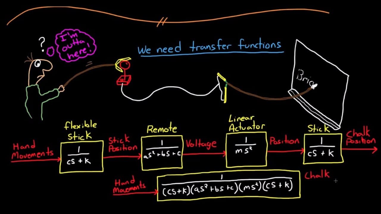
• Connected component models can be combined by multiplying their transfer functions. In the chalkboard example, models for flexible sticks, a remote control, and linear actuators combine into a single plant model relating hand motion to chalk position.
• The chalkboard arrangement is a closed-loop system because the student visually senses the chalk position, compares it with the desired writing, interprets the error, and generates hand commands. Removing the student would require replacing these feedback functions with automatic control.

Questions & Answers

Q: What is a transfer function in control systems?

A transfer function is the Laplace transform of the impulse response of a linear, time-invariant system when its initial conditions are set to zero. It represents the system as an S-domain black box that maps an input signal to a modified output approximating the modeled physical process.

Q: Why are transfer functions useful for control-system modeling?

Transfer functions let control engineers characterize filters, actuators, flexible elements, and other components separately. They can then combine those models algebraically to understand the behavior of the complete connected system and simplify control-system design and analysis.

Q: How does the Laplace transform simplify convolution?

In the time domain, the output is the convolution of the arbitrary input U of t and the impulse response G of t. The Laplace transform maps these signals into the S domain, where the convolution becomes ordinary multiplication of U of s and G of s.

Q: How does an impulse response characterize an LTI system?

An arbitrary input can be divided into infinitely many scaled and time-shifted impulses. Because the system is linear and time invariant, its corresponding impulse responses can be scaled, shifted, and summed to determine the output, with that sum represented by the convolution integral.

Q: How is a transfer function derived from an equation of motion?

Take the Laplace transform of the equation of motion, set the initial conditions to zero, and solve algebraically for the transformed output relative to the transformed input. Setting the initial position and velocity to zero removes their terms from the transformed derivatives.

Q: What is the transfer function of the mass-and-spring example?

The example uses an equation of motion in which mass times acceleration plus spring constant times position equals the input forcing function. With zero initial conditions, its transfer function is 1 divided by ms squared plus K.

Q: How are component transfer functions combined into a plant model?

Transfer functions for sequential components are multiplied in the S domain. In the lecture’s chalkboard example, the models for a flexible stick, remote control, linear actuators, and a second flexible stick combine into an overall plant model relating hand movement to chalk position.

Q: Why is the chalkboard arrangement a closed-loop control system?

The student’s eyes sense the chalk position, which is compared with the desired writing. The student interprets the error and produces corrective hand commands, forming a feedback loop; removing the student would require replacing those feedback functions with automatic control.

Summary & Key Takeaways

• Transfer functions provide compact S-domain models of linear, time-invariant systems under zero initial conditions. A transfer function is the Laplace transform of the system's impulse response. It acts like a black box that accepts an input and produces a modified output approximating the behavior of a real physical process.

• An arbitrary input can be represented as scaled and time-shifted impulses. In the time domain, the resulting output is calculated by convolving that input with the impulse response. Applying the Laplace transform replaces this difficult convolution integral with ordinary multiplication of the transformed input and the transfer function in the S domain.

• For a mass and spring system, transforming the equation of motion with zero initial conditions produces the transfer function 1 divided by ms squared plus K. Connected components can be modeled separately and multiplied together, producing an overall plant transfer function from hand motion to chalk position in the lecture's illustrative system.