General Relativity Lecture 10

TL;DR

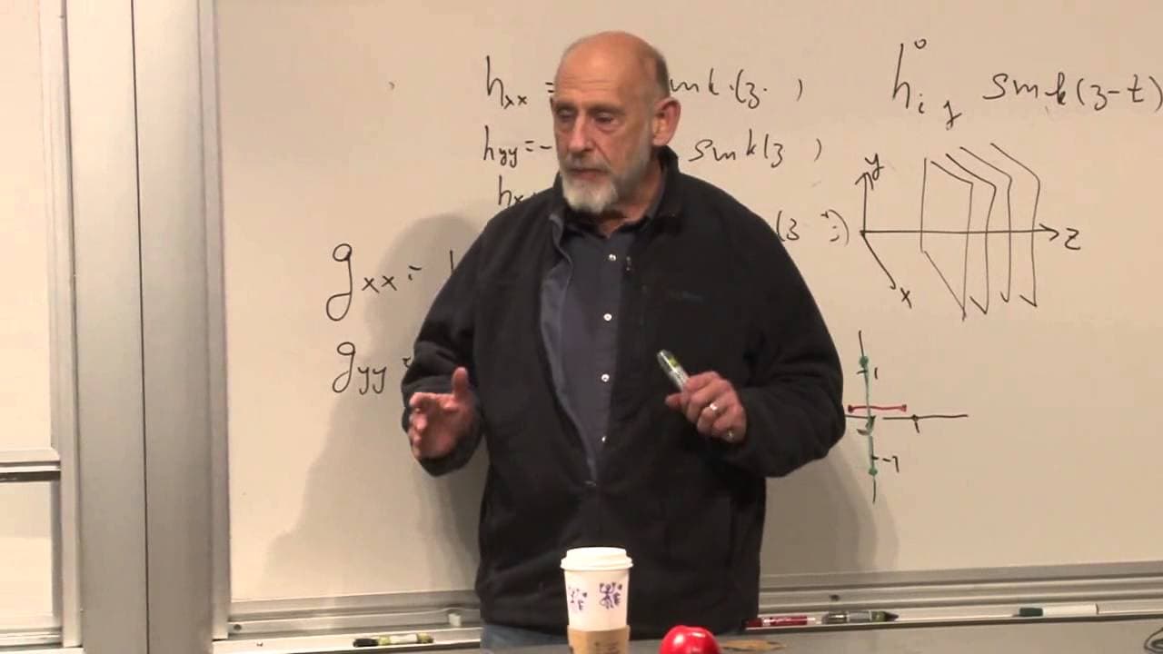
Einstein's equations become gravitational wave equations when the metric is written as flat spacetime plus a small correction, h_mu_nu, and every term quadratic in that correction is discarded. In vacuum, tracing the field equations gives R equals zero, while linearizing the Ricci tensor leaves second derivatives of h with respect to position and time. Read on to follow each step from the vacuum equation to weak gravitational waves.

Transcript

Stanford University so the questions that were asked to me tonight are more or less by accident they exactly the ones that I want to address tonight weak gravitational fields linearity versus nonlinearity um and gravitational waves let's again working out the equations of general relativity is always unpleasant and we're not going to do it on the B... Read More

Key Insights

• Smallness creates a hierarchy: The weak-field approximation does not set the disturbance itself to zero. It keeps contributions that are linear in h_mu_nu while neglecting contributions containing two small factors. This distinction preserves the leading change in the metric, which carries the wave, while removing the nonlinear terms that make the complete Einstein equations difficult to solve.
• Vacuum removes the source term: The lecture studies a region without matter, so there is no energy momentum tensor on the right side of Einstein's equations. The resulting equation constrains the spacetime curvature directly. This is appropriate for radiation observed far from the complicated system that generated it, where the wave can be weak and the local region can be treated as vacuum.
• Tracing gives the first simplification: Contracting R_mu_nu minus one-half g_mu_nu R equals zero shows that the scalar curvature R vanishes. Substituting that result back into the original equation removes its second term. The gravitational perturbation must consequently satisfy the simpler vacuum requirement that the Ricci tensor itself be zero.
• Equilibrium means time independence: Before discussing fluctuations, Susskind selects a background that does not change with time and contains no matter. Empty flat spacetime satisfies both conditions and has no curvature. It provides the uncomplicated reference geometry needed to separate a small, variable gravitational disturbance from the fixed metric around which the equations are expanded.
• Coordinates affect metric appearance: Flatness does not require the metric components to look identical in every coordinate system. Polar or other curved coordinates can give a flat geometry a less simple metric. The relevant property is that coordinates can be chosen in which flat spacetime is represented by eta_mu_nu, making the weak-field expansion especially transparent.
• The background solves Einstein's equations: Eta_mu_nu is not merely a convenient notation for comparison. In the selected coordinates it represents a spacetime with no curvature, so it satisfies the vacuum field equations directly. Starting with an exact equilibrium solution ensures that the remaining equation isolates the behavior of the added perturbation rather than an error in the background.
• Distance weakens emitted radiation: A binary pulsar can involve strong gravity and strong gravitational waves near the source. Susskind's approximation concerns a sufficiently distant region, where the emitted gravitational radiation has become weak. The same physical source can therefore require nonlinear treatment nearby while permitting a linear weak-field treatment far away.
• The perturbation carries variation: Eta_mu_nu consists of constant components, whereas h_mu_nu generally changes with the spacetime coordinates. Its dependence on both position and time is what allows the correction to describe a wave. The decomposition separates the unchanging flat background from the changing part whose motion the linearized equations are intended to determine.
• Constant backgrounds have zero derivatives: Differentiating eta_mu_nu gives zero because its components are constants. When derivatives of the full metric are calculated, only derivatives of h_mu_nu remain. This makes each leading Christoffel symbol proportional to a derivative of the perturbation and begins the conversion of geometric curvature expressions into differential equations for h.
• Curvature introduces second derivatives: The Ricci tensor contains a derivative of a Christoffel symbol, while a Christoffel symbol already contains a metric derivative. Its linear contribution therefore contains second derivatives of h_mu_nu. Those derivatives include changes with position and time, providing the differential structure associated with propagation through spacetime.
• Connection products are nonlinear: The Ricci tensor also contains products of Christoffel symbols. Since each leading Christoffel symbol is proportional to a derivative of h, their product contains two small factors and is quadratic in the perturbation. The weak-field rule removes these products, leaving the part of curvature that depends linearly on h and its derivatives.
• Wave behavior emerges after linearization: Once quadratic contributions are discarded, the vacuum equation is composed of second derivatives of h_mu_nu with respect to space and time. Susskind identifies equations of this form, particularly in relativity, as wave equations. Gravitational waves therefore appear as small, coordinate-dependent fluctuations of the metric propagating on a flat spacetime background.

Questions & Answers

Q: How do Einstein's equations become gravitational wave equations in General Relativity Lecture 10?

Begin with the vacuum field equation, R_mu_nu minus one-half g_mu_nu R equals zero, and take its trace to obtain R equals zero. Write the true metric as eta_mu_nu plus a small, position-dependent and time-dependent correction h_mu_nu. When the Ricci tensor is calculated, keep terms linear in h and discard products containing two small factors. The surviving vacuum equation contains second derivatives of h with respect to position and time, which gives it the form of a wave equation.

Q: What does weak gravitational wave mean?

A weak gravitational wave has an amplitude small enough that higher-order contributions can be ignored. The metric correction h_mu_nu is retained because it is the leading disturbance, but terms proportional to its square or to products of small derivatives are dropped. This converts the nonlinear calculation into a linear approximation. The approximation can apply far from a source even when gravity and radiation are strong near that source.

Q: What are Einstein's vacuum field equations?

Without matter or an energy momentum tensor, the equation is R_mu_nu minus one-half g_mu_nu R equals zero. Taking the trace of both sides shows that the scalar curvature R equals zero. Substitution then eliminates the term containing g_mu_nu R and leaves R_mu_nu equals zero. This simpler condition is used to derive the equation governing the weak metric perturbation.

Q: Why is flat spacetime used as the background?

The calculation begins with an equilibrium that has no time dependence and no matter. Empty flat spacetime meets those conditions and has no curvature, so it solves the vacuum Einstein equations. In an appropriate coordinate system, its metric is written as eta_mu_nu. Using this exact and simple solution makes it possible to describe weak gravity as a small fluctuation around equilibrium.

Q: What is h_mu_nu in the weak-field approximation?

H_mu_nu is the small correction added to the flat-spacetime metric, so the full metric is eta_mu_nu plus h_mu_nu. Its components are much smaller than the components appearing in the background metric. Unlike eta_mu_nu, it can vary with position and time. That variation lets h_mu_nu represent the gravitational disturbance whose equation of motion is being calculated.

Q: Why can quadratic terms in h_mu_nu be ignored?

The approximation treats h_mu_nu and its smooth derivatives as small quantities. A term containing one such factor is kept, while a product containing two small factors is higher order and is neglected. For example, Christoffel-times-Christoffel terms contain two derivatives of h and are therefore quadratic in the perturbation. Removing them isolates the leading, linear behavior of a weak gravitational field.

Q: How do Christoffel symbols contribute to the wave equation?

A Christoffel symbol contains the inverse metric multiplied by a derivative of the metric. Because eta_mu_nu is constant, its derivatives vanish, leaving the leading Christoffel contribution proportional to derivatives of h_mu_nu. Differentiating that Christoffel symbol inside the Ricci tensor produces second derivatives of h. Products of two Christoffel symbols are quadratic and are discarded in the weak-field approximation.

Q: Why can strong sources still produce weak waves?

Susskind uses a rotating binary pulsar as an example of a complicated source. Close to it, the gravitational field and even the gravitational waves may be strong. Far enough away, however, the radiation produced by the system becomes very weak. In that distant region, the metric can be represented as flat spacetime plus a small perturbation, making the linear approximation applicable.

Summary

In this video, the lecturer discusses weak gravitational fields, linearity versus non-linearity, and gravitational waves. They start by explaining that although working out the equations of general relativity is complicated and not suitable for the blackboard, the principles are straightforward. The lecturer goes on to describe weak gravitational waves as small amplitude fluctuations in the gravitational field, and explains how to make approximations when solving for these waves. They then discuss equilibrium situations and how the metric of flat space can be chosen and represented in different coordinates. Moving on to the equations of motion, the lecturer presents a schematic view of the equations, explaining that they have a relatively simple form and resemble wave equations. Finally, they discuss the nature of gravitational waves, the transversality of the fields, and the effect of these waves on the metric tensor.

Questions & Answers

Q: How can the equations of general relativity be summarized?

The equations of general relativity are typically unpleasant to work with on the blackboard, but they can be summarized by the principles and solutions obtained from solving the equations.

Q: What are weak gravitational waves?

Weak gravitational waves refer to small amplitude fluctuations in the gravitational field. They are characterized by the amplitudes of the waves being small enough to make approximations.

Q: Explain the concept of equilibrium situations.

Equilibrium situations describe solutions with no time dependence and no matter on the right-hand side of the equations. In other words, it is a situation of empty space with no curvature or interesting gravitational fields.

Q: How does the metric of flat space depend on coordinates?

The metric of flat space depends on the coordinates used. While one commonly used metric is the Kronecker Delta, there can be other metrics depending on the choice of coordinates. The special feature of flat space is that there are coordinates in which the metric has a simple form.

Q: What are the components of the metric tensor of flat space?

The metric tensor of flat space can be written as a matrix of components: 1 -1 -1 -1 for the first row and column, followed by 0 0 0 0, 0 0 1 0, and 0 0 0 1.

Q: What is the significance of weak gravitational waves being small?

The smallness of weak gravitational waves allows for approximations to be made, such as ignoring higher order terms. This simplifies the equations and makes them more manageable to work with.

Q: How can the equations of motion for weak gravitational waves be summarized?

The equations of motion for weak gravitational waves have a relatively simple form and resemble wave equations. They can be written using second derivatives of the metric tensor and involve the Christoffel symbol, Ricci tensor, and more.

Q: How does the metric tensor change with gravitational waves?

The metric tensor of flat space is modified by gravitational waves, represented by a small correction term called H_mu_nu. This term depends on the position and time coordinates, and describes the wave field.

Q: What are the constraints on gravitational waves derived from Einstein's field equations?

The constraints on gravitational waves require the transversality of the fields, meaning that the time and Z components of H must be zero. Additionally, the trace of H_ij must be zero.

Q: Can you provide an example of the components of the metric tensor for a gravitational wave?

For gravitational waves propagating along the Z axis, the components of the metric tensor that are allowed to be nonzero are H_ij times sine(KX) times sine(KZ-T), where K represents the wave number. The other components are set to zero.

Takeaways

Gravitational waves are small amplitude fluctuations in the gravitational field. They can be approximated as weak gravitational waves, allowing for simplifications in the equations of motion. The metric tensor of flat space can be modified by gravitational waves, characterized by a small correction term called H_mu_nu. The constraints on gravitational waves include transversality of the fields and the trace of H_ij being zero. Gravitational waves can cause tidal forces and deformations in physical objects, making them an interesting field of study.

Summary & Key Takeaways

• Introducing the weak-field problem: Susskind frames General Relativity Lecture 10 around weak gravitational fields, linearity versus nonlinearity, and gravitational waves. Because a complete blackboard derivation would be lengthy and not especially illuminating, he focuses on the governing principles and the form of the resulting equations. Weak gravitational waves have amplitudes small enough to justify an expansion in which higher-order terms, including the amplitude squared, are ignored.

• Simplifying the vacuum equations: With no matter or energy momentum tensor, Einstein's equations are R_mu_nu minus one-half g_mu_nu R equals zero. Taking the trace shows that the scalar curvature R equals zero. The second term can therefore be removed, leaving the simpler condition R_mu_nu equals zero. This vacuum equation supplies the starting point for finding an equation governing a small gravitational disturbance.

• Choosing the equilibrium background: The perturbation is defined around an equilibrium solution with no time dependence and no matter. Susskind identifies that situation as empty flat spacetime, with no curvature or interesting gravitational field. Although a metric depends on the coordinates selected, flat spacetime permits coordinates in which the metric has the simple form eta_mu_nu. This constant metric solves the vacuum field equations because all of its curvature vanishes.

• Adding a small disturbance: Far from a complicated source such as a rotating binary pulsar, gravitational radiation becomes weak even if the nearby field is strong. In suitable coordinates, the true metric is written as eta_mu_nu plus the small correction h_mu_nu. Its components are much smaller than those of the flat metric. Unlike constant eta_mu_nu, h_mu_nu depends on position and time, allowing it to represent a propagating disturbance.

• Recovering the wave equation: The perturbed metric is inserted into the Ricci tensor, and the vacuum condition is imposed. Derivatives of constant eta_mu_nu vanish, so the Christoffel symbols are proportional to derivatives of h. The Ricci tensor contains derivatives of Christoffel symbols and products of Christoffel symbols. Dropping the quadratic products leaves only terms containing second derivatives of h, producing the linear equations identified as gravitational wave equations.