No full solar-time slope in Japan's 2021 prefecture mean wake times

A short research note on weekday mean wake times by prefecture in Japan's 2021 Survey on Time Use and Leisure Activities, viewed against longitude

Japan runs on a single time zone, so every clock in the country shows the same time, but local mean solar time advances by about 4 minutes for each degree east (at the same latitude on the same day, sunrise also comes that much earlier). Japan is divided into 47 prefectures, its top-level administrative units. Excluding Okinawa, the population centroids of the other 46 prefectures span about 12 degrees of longitude, from 129.8 degrees east (Nagasaki) to 141.9 degrees east (Hokkaido), a difference of about 48 minutes in mean solar time between the western and eastern ends. Are published prefecture mean wake times earlier in the east?

Studies abroad have reported, with individual data, a slope towards earlier timing in the east. In Germany, a chronotype measure built from sleep timing on free days was about 4 minutes earlier per degree east, and the association weakened in larger cities (Roenneberg et al. 2007). In the American Time Use Survey, in 3 of the 4 time zones, the midpoint of weekend sleep was 1.2 to 2.4 minutes later per degree west (Fischer and Lombardi 2022). Czechia also shows a weak slope in the same direction (Sládek et al. 2020). On the other hand, a study comparing term time and vacation in 112 adolescents in Singapore found that their internal clocks shifted to fit early school hours (Charoenthammanon and Gooley 2025), so results are not uniform across measures and populations.

Data and method

The outcome is the weekday mean wake time by prefecture (age 10 and over, both sexes combined, all areas) from the 2021 Survey on Time Use and Leisure Activities of the Statistics Bureau of Japan. The survey covers household members aged 10 and over; residents of social welfare facilities and hospital inpatients, among others, are outside its scope. Each respondent recorded activities over two consecutive designated days between 16 and 24 October 2021. In the survey's definition, the wake time is the end of the first sleep episode that begins before noon (12:00) on the first designated day and lasts more than 60 minutes; non-sleep activities of 30 minutes or less between two sleep episodes count as continued sleep. The published mean is taken over the people who have a wake time under this definition (99.3% of the population aged 10 and over on weekdays nationally), not over everyone. Each prefecture's position is the longitude and latitude of its 2020 population centroid as published by the Statistics Bureau. All values used are listed in Appendix B.

Before the main estimate was computed, the model and the rules for reading its result were written down in an internal analysis plan dated 2026-10-24 (dated in private version control, not publicly registered). Some raw values had been seen while checking the layout of the tables, so the plan was not blind. Appendix A gives an English translation of its decision rules. The main model is an unweighted ordinary least-squares regression of mean wake time (minutes) on longitude, latitude, and the share of the population living in census-defined Densely Inhabited Districts (DIDs). The DID share is computed from the weekday estimated population in the same table, as DID population divided by total population. Intervals use heteroskedasticity-robust standard errors (HC3) and a t distribution with 42 degrees of freedom. Okinawa lies more than 2 degrees of longitude away from the others and could move the slope substantially on its own, so the plan excluded it from the main analysis (including it changes the slope from +0.21 to +0.01 minutes per degree, 95% CI -1.07 to +1.09).

The benchmarks are two idealized lines. If waking followed local mean solar time exactly, the slope would be -4 minutes per degree of longitude (earlier in the east); if it were set by clock time alone, 0 minutes. Age structure and industry can also vary with longitude, so neither line represents a mechanism.

Results

The longitude slope was +0.21 minutes per degree, with a 95% confidence interval from -0.84 to +1.27 minutes. As a ratio to -4 minutes, this is -5.3% (-31.7% to +21.1%); this ratio is not the share of people who follow the sun. Both -4 minutes and half of it, -2 minutes, lie outside the interval. The interval does, however, extend 0.84 minutes per degree in the solar direction (about 20% of -4 minutes), so a small solar-direction slope is not excluded. In the same model, a 10-percentage-point higher DID share was associated with a mean wake time about 3 minutes later (+30.5 minutes per unit share, 95% CI +19.5 to +41.6). The latitude coefficient was -1.40 minutes per degree north (-2.99 to +0.18).

The Statistics Bureau also publishes the standard error (SE) of each prefecture mean (1 to 7 minutes for weekday wake time). Two checks added after the plan use these SEs. A weighted version of the main regression, with weights 1/SE² and an HC3 interval computed on the weighted regression, gives +0.52 minutes per degree (-0.85 to +1.89). A random-effects meta-regression with the same regressors, the between-prefecture variance estimated by restricted maximum likelihood (REML) and Knapp-Hartung intervals with 42 degrees of freedom, gives +0.28 minutes (-0.55 to +1.10). Both intervals exclude -2 and -4.

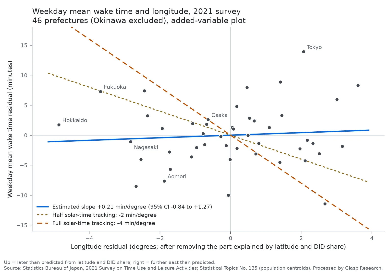
Figure: added-variable (partial regression) plot, 46 prefectures. The parts of wake time and of longitude explained by latitude and DID share are removed, and the residuals are plotted. The blue line has the same slope as the estimated longitude coefficient, +0.21 minutes per degree. The dashed lines show full (-4 minutes per degree) and half (-2) solar-time tracking, drawn through the origin for comparison.

Secondary analyses listed in the plan

The plan also listed secondary analyses that do not change how the main result is read. Those that can be computed from the same published table (Table 2-1, 2016 and 2021 surveys) are below; longitude and latitude are the 2020 centroids in both years, and Okinawa is excluded.

• S7: Outcome and model: 2016 survey, weekday, main model (2016 DID share); Longitude slope (min/degree): -0.46; 95% CI: -1.34 to +0.42

• S2: Outcome and model: 2021 Saturday, main model; Longitude slope (min/degree): +0.68; 95% CI: -0.46 to +1.83

• S2: Outcome and model: 2021 Sunday, main model; Longitude slope (min/degree): +1.07; 95% CI: -0.28 to +2.42

• S2: Outcome and model: 2016 Saturday, main model; Longitude slope (min/degree): +0.42; 95% CI: -0.84 to +1.68

• S2: Outcome and model: 2016 Sunday, main model; Longitude slope (min/degree): -0.26; 95% CI: -1.32 to +0.80

• S1: Outcome and model: 2021 weekday, inside DIDs only, longitude and latitude; Longitude slope (min/degree): +0.51; 95% CI: -1.07 to +2.09

• S1: Outcome and model: 2021 weekday, outside DIDs only, longitude and latitude; Longitude slope (min/degree): +0.39; 95% CI: -0.50 to +1.29

• S1: Outcome and model: 2016 weekday, inside DIDs only, longitude and latitude; Longitude slope (min/degree): -0.78; 95% CI: -1.96 to +0.39

• S1: Outcome and model: 2016 weekday, outside DIDs only, longitude and latitude; Longitude slope (min/degree): +0.62; 95% CI: -0.05 to +1.30

Every one of these intervals includes 0 and excludes -2 and -4. The 2016 weekday slope has the opposite sign to 2021, so the sign of the slope is not stable across the two years; what is stable is that neither year's interval reaches -2. The plan's predictions that weekends and areas outside DIDs would show more negative slopes were not borne out, except for a 0.12 minutes per degree difference in the expected direction between the 2021 inside-DID and outside-DID slopes. The plan also listed bedtime, the 2006 and 2011 surveys, employment status and a permutation test; these use other tables or were revised after the plan, and are not reported in this note.

Check allowing for correlation between nearby prefectures (added after the plan)

The HC3 interval assumes that the errors of different prefectures are independent. If nearby prefectures resemble each other, the interval may be too narrow. After the plan, Conley standard errors based on the distance between population centroids were therefore computed. Errors may correlate more for closer pairs of prefectures (Bartlett kernel, weight = 1 - distance / cutoff distance), and pairs farther apart than the cutoff get weight 0. The slope stays at +0.21 minutes; only the interval changes.

• Main model, HC3 (as planned): 95% CI (minutes per degree): -0.84 to +1.27; -2 minutes: outside; -4 minutes: outside

• Main model, Conley 100 km: 95% CI (minutes per degree): -0.65 to +1.08 (HC3-scaled residuals: -0.79 to +1.22); -2 minutes: outside; -4 minutes: outside

• Main model, Conley 200 km: 95% CI (minutes per degree): -0.53 to +0.96 (HC3-scaled residuals: -0.66 to +1.08); -2 minutes: outside; -4 minutes: outside

• Main model, Conley 300 km: 95% CI (minutes per degree): -0.42 to +0.84 (HC3-scaled residuals: -0.53 to +0.96); -2 minutes: outside; -4 minutes: outside

• Main model, Conley 500 km: 95% CI (minutes per degree): -0.27 to +0.70 (HC3-scaled residuals: -0.37 to +0.79); -2 minutes: outside; -4 minutes: outside

• Main model plus region fixed effects (slope -0.46, HC3, 35 degrees of freedom; see Appendix C): 95% CI (minutes per degree): -3.26 to +2.33; -2 minutes: inside; -4 minutes: outside

At each of the 4 cutoffs, the Conley interval was narrower than the HC3 interval, and -2 and -4 lay outside it. With only 46 points, standard errors of this kind can come out too small, and the t(42) reference distribution does not reflect a spatially reduced effective sample size; at 300 km the weight matrix is also not positive semidefinite (Appendix C). The conclusion therefore keeps the wider HC3 interval. This check supports only the statement that, with the Bartlett kernel and the 4 cutoff distances tried here, allowing correlation between nearby prefectures did not widen the interval to -2 minutes. It does not show robustness to other kernels, other cutoffs, or spatial correlation in general.

Within regions alone, half tracking cannot be ruled out

The conclusions so far come from a model that also uses differences in longitude between regions. As in the last row of the table above, when fixed effects for the regions (Tohoku, Kanto, Chubu, Kinki, Chugoku, Shikoku, Kyushu; Hokkaido, a region of a single prefecture, is dropped, leaving 45 prefectures) are added and only differences in longitude within the same region are used, the slope is -0.46 minutes (-3.26 to +2.33): the interval widens greatly and -2 minutes falls inside it (-4 minutes stays outside). The east-west extent within a region is narrow, so this model cannot tell whether waking tracks solar time halfway.

The plan also refits the main model leaving out one region at a time. Leaving out the Kanto region (the seven prefectures from Ibaraki to Kanagawa, including Tokyo) changes the point estimate from +0.21 to -0.08 (95% CI -1.43 to +1.27). Both estimates are close to 0, their intervals overlap almost entirely, and -2 minutes stays outside, so the interval-based reading does not change. Because the plan's rule says that a sign change when one region is left out must be reported as a result that depends on that region, with the conclusion weakened, this note describes the slope only as "close to 0" and not as positive.

The 2021 survey days came just after the COVID-19 state of emergency and the priority measures to prevent its spread had ended in all areas of Japan at the end of September 2021, and the Statistics Bureau notes that the allocation of daily time changed compared with the 2016 survey (Summary of Results, 2021). The 2016 weekday estimate is reported above; surveys before 2016 are not analyzed in this note.

What this note does not say

• It says nothing about individual waking or internal clocks. It compares the published means of 46 prefectures.

• It shows neither a mechanism such as "people wake by the clock" nor a causal effect of longitude on waking.

• It measures something different from the studies abroad. Most of those use individuals' sleep timing on free days; this note uses weekday prefecture mean wake times.

• It covers the 2021 survey, with the 2016 survey as a secondary check; earlier surveys are not analyzed here.

• The point estimate for latitude points to slightly earlier mean waking in more northern prefectures, but its interval includes 0. A north-south difference is not a finding of this note.

What can be said is this: for the published prefecture mean wake times in the 2021 survey, the model fixed in advance did not show a slope corresponding to full solar-time tracking. The data were also inconsistent with tracking solar time halfway or more, but only when differences in longitude between regions are used; differences within the same region alone cannot rule out half tracking.

Disclosure

The text was drafted with AI assistance (Anthropic Claude) and checked against the cited sources and the replication files. It was reviewed by an AI reviewer (OpenAI Codex). No Glasp user data were used. The work received no external funding, and the authors know of no conflicts of interest.

Replication files (code and data): deposited with this note. https://doi.org/10.5281/zenodo.23838809

Appendix A: decision rules of the internal analysis plan (translated from the Japanese document dated 2026-10-24)

The main model, the sample (46 prefectures excluding Okinawa), and HC3 with a t distribution (n - 4 degrees of freedom) were fixed in advance exactly as described in the text. The rules for reading the result are translated below.

Decide by the 95% interval of the main b.

• Excludes 0, and b < 0: "Prefecture mean waking follows the direction of the sun." Report the following share b/(-4). If the interval also includes -4, add "indistinguishable from full following".

• Includes 0, does not include -4: "Full sun-following can be rejected." If the lower end of the interval is above -2, write "half-following can also be rejected; close to the clock".

• Includes both 0 and -4: stopping condition 1.

• Excludes 0, and b > 0: write plainly "earlier in the west (opposite to the prediction)", and name no cause.

In every case, keep to "prefecture averages" and do not write about individual internal clocks (ecological comparison).

In falsification check R2, if leaving out 1 region changes the sign of the main b, write "a result that depends on that region" and weaken the conclusion (do not stop).

The interval obtained here falls under the second rule. This note does not use the phrase "close to the clock", and writes only what the interval rules out. The "following share" is called "the ratio to -4 minutes" in the text. The SE-weighted checks, the Conley standard errors and the region fixed effects are not in the plan; they were added afterwards.

Appendix B: data (values used in the main model)

One row per prefecture. Okinawa (code 47) is excluded from the main model and used only for the check that includes it. Prefecture names are romanized. The columns and their sources:

• lon, lat: east longitude and north latitude (degrees) of the 2020 population centroid, converted to degrees from the degrees, minutes and seconds in Table 2-3 (population centroids of prefectures, World Geodetic System) of Statistical Topics No. 135.

• did: DID share. From the 2021 Average Time of Day volume, Table 2-1 (e-Stat statInfId 000032224371): weekday estimated population, age 10 and over, both sexes, inside DIDs divided by all areas.

• wake: weekday mean wake time (minutes after 0:00; 393 is 6:33). Same Table 2-1, weekday, age 10 and over, both sexes, all areas (the "total" category of the DID classification).

• se: published standard error of that mean (minutes, integer). Weekday wake time in Table 15 (standard errors of mean time of day by day of the week, all Japan and prefecture, and type of activity) of the 2021 Standard Error Rates of Main Items. Not used in the main model; used only in the SE-weighted checks.

code,pref,lon,lat,did,wake,se
1,Hokkaido,141.86827,43.07784,0.8145,393,1
2,Aomori,140.92600,40.70856,0.5156,377,2
3,Iwate,141.28381,39.50846,0.3563,381,2
4,Miyagi,140.95415,38.33554,0.6780,391,5
5,Akita,140.26791,39.70527,0.3534,381,4
6,Yamagata,140.16406,38.41349,0.5784,387,2
7,Fukushima,140.45599,37.41010,0.5129,386,4
8,Ibaraki,140.27279,36.21035,0.4191,395,2
9,Tochigi,139.83264,36.53015,0.5064,386,3
10,Gunma,139.14162,36.35804,0.4611,387,2
11,Saitama,139.58162,35.92343,0.8442,396,3
12,Chiba,140.07836,35.67802,0.7584,396,2
13,Tokyo,139.64186,35.68741,0.9909,419,2
14,Kanagawa,139.51321,35.45479,0.9587,403,3
15,Niigata,138.89941,37.63638,0.5350,390,3
16,Toyama,137.16346,36.71687,0.4067,384,1
17,Ishikawa,136.64389,36.61884,0.6058,394,1
18,Fukui,136.17296,35.95856,0.4594,388,2
19,Yamanashi,138.61651,35.62751,0.3131,390,4
20,Nagano,138.11490,36.26294,0.4145,382,2
21,Gifu,136.89505,35.46547,0.4569,390,2
22,Shizuoka,138.30848,34.92531,0.6532,384,2
23,Aichi,137.00076,35.08707,0.8096,397,2
24,Mie,136.52191,34.75567,0.5280,395,4
25,Shiga,136.06697,35.11088,0.5519,400,3
26,Kyoto,135.68328,35.01032,0.8736,404,2
27,Osaka,135.53092,34.66620,0.9647,408,5
28,Hyogo,135.07630,34.78338,0.7805,398,3
29,Nara,135.77066,34.59073,0.6644,399,4
30,Wakayama,135.31980,34.09722,0.4203,398,1
31,Tottori,133.77894,35.45769,0.4298,389,7
32,Shimane,132.73187,35.27619,0.2901,387,3
33,Okayama,133.85251,34.68318,0.5216,388,3
34,Hiroshima,132.72160,34.42742,0.7514,395,1
35,Yamaguchi,131.50343,34.07232,0.5285,384,3
36,Tokushima,134.46186,34.04951,0.4019,391,4
37,Kagawa,133.96431,34.27796,0.3250,387,3
38,Ehime,132.87651,33.79827,0.5365,391,3
39,Kochi,133.46853,33.46475,0.4967,397,3
40,Fukuoka,130.56557,33.59884,0.7749,408,4
41,Saga,130.19398,33.28864,0.3428,395,3
42,Nagasaki,129.83473,32.95941,0.5066,392,1
43,Kumamoto,130.68642,32.73900,0.5215,391,2
44,Oita,131.53129,33.26371,0.5689,389,3
45,Miyazaki,131.36469,32.02187,0.5022,384,2
46,Kagoshima,130.48724,31.35654,0.4800,390,2
47,Okinawa,127.53713,26.16176,0.7221,392,2

The secondary analyses use, in addition, the 2016 and 2021 Table 2-1 values for weekdays, Saturdays and Sundays, inside and outside DIDs, which are in the replication files (with the script that extracts them from the two e-Stat tables).

Appendix C: model and code for reproduction

• Sample: 46 prefectures excluding Okinawa.

• Model: wake = a + b × lon + c × lat + d × did + error. Unweighted ordinary least squares (OLS).

• Interval: HC3 (robust standard errors with residuals multiplied by 1 / (1 - h), where h is the leverage), with the 97.5% point of the t distribution with 46 - 4 = 42 degrees of freedom, 2.0181.

• Post hoc Conley standard errors: distance is the great-circle distance between population centroids (Earth radius 6371 km). Bartlett kernel weight max(0, 1 - distance / cutoff), cutoffs 100, 200, 300 and 500 km. The weight for a prefecture paired with itself is 1. Two variants: one using the residuals as they are, and one multiplying them by 1 / (1 - h) as in HC3. Intervals use the same t(42). At 300 km the weight matrix is not positive semidefinite (smallest eigenvalue -0.018), but the variance of the slope was positive.

• Post hoc region fixed effects: 8 regions (Hokkaido 1, Tohoku 2 to 7, Kanto 8 to 14, Chubu 15 to 23, Kinki 24 to 30, Chugoku 31 to 35, Shikoku 36 to 39, Kyushu 40 to 46; numbers are codes). Hokkaido is a region of one prefecture: with its own dummy its leverage is 1, so the HC3 term is undefined, and it carries no within-region information. It is therefore dropped, and fixed effects for the seven remaining regions (the intercept plus six region indicators, with Tohoku as the reference) are fitted on 45 prefectures, with HC3 and the 97.5% point of t(35), 2.0301 (45 observations, 10 parameters).

• Post hoc SE-weighted checks: (1) weighted least squares with weights 1/SE², done as OLS on rows multiplied by 1/SE, with HC3 on that transformed regression; (2) random-effects meta-regression with sampling variance SE², between-prefecture variance tau² by REML (grid search from 0 to 200 in steps of 0.01), and the Knapp-Hartung variance q × (X'WX)⁻¹ with q = Σ w e² / (n - 4), not truncated at 1, and t(42).

Saving the Appendix B block as a file named h2_data.csv and running the following code in the same place (Python 3 and numpy only) produces the reported model estimates and confidence intervals other than those in the secondary-analysis table and the figure, which come from the scripts in the replication files.

import numpy as np

d = np.genfromtxt("h2_data.csv", delimiter=",", names=True, dtype=None, encoding="utf-8")
d = d[d["code"] != 47]                      # 46 prefectures, Okinawa excluded
n = len(d)
X = np.column_stack([np.ones(n), d["lon"], d["lat"], d["did"]])
y = d["wake"].astype(float)
T42 = 2.0181                                # 97.5% point of t (42 degrees of freedom)

def fit(X, y):
    A = np.linalg.inv(X.T @ X)
    b = A @ X.T @ y
    e = y - X @ b
    h = np.einsum("ij,jk,ik->i", X, A, X)
    return b, e, h, A

def sandwich(X, u, A, W=None):
    s = X * u[:, None]
    M = s.T @ s if W is None else s.T @ W @ s
    return np.sqrt(np.diag(A @ M @ A))

b, e, h, A = fit(X, y)
se = sandwich(X, e / (1 - h), A)            # HC3
print(f"b = {b[1]:+.2f}, 95% CI {b[1]-T42*se[1]:+.2f} to {b[1]+T42*se[1]:+.2f}")

# Post hoc check: Conley standard errors (Bartlett kernel, great-circle distance between centroids)
la, lo = np.radians(d["lat"]), np.radians(d["lon"])
a = (np.sin((la[:, None]-la)/2)**2
     + np.cos(la[:, None])*np.cos(la)*np.sin((lo[:, None]-lo)/2)**2)
D = 2 * 6371 * np.arcsin(np.sqrt(a))        # km
for cut in (100, 200, 300, 500):
    W = np.clip(1 - D / cut, 0, None)
    for name, u in (("plain", e), ("HC3-scaled", e / (1 - h))):
        s = sandwich(X, u, A, W)[1]
        print(f"Conley {cut} km {name}: {b[1]-T42*s:+.2f} to {b[1]+T42*s:+.2f}")

# Post hoc check: region fixed effects (code breaks Hokkaido|Tohoku|Kanto|Chubu|Kinki|Chugoku|Shikoku|Kyushu)
reg = np.digitize(d["code"], [2, 8, 15, 24, 31, 36, 40])
r = reg > 0                                 # drop Hokkaido, a one-prefecture region (leverage 1)
F = np.column_stack([X[r]] + [(reg[r] == k).astype(float) for k in range(2, 8)])
bf, ef, hf, Af = fit(F, y[r])
sf = sandwich(F, ef / (1 - hf), Af)[1]      # HC3, 45 - 10 = 35 df, 97.5% point of t 2.0301
print(f"region FE: b = {bf[1]:+.2f}, 95% CI {bf[1]-2.0301*sf:+.2f} to {bf[1]+2.0301*sf:+.2f}")

# Ratio to -4, DID share and latitude coefficients of the main model
lo_b, hi_b = b[1] - T42*se[1], b[1] + T42*se[1]
print(f"ratio to -4: {100*b[1]/-4:+.1f}% ({100*hi_b/-4:+.1f}% to {100*lo_b/-4:+.1f}%)")
for k, name in ((3, "DID share"), (2, "latitude")):
    print(f"{name}: {b[k]:+.2f}, 95% CI {b[k]-T42*se[k]:+.2f} to {b[k]+T42*se[k]:+.2f}")

# Kanto (codes 8 to 14) left out: 39 prefectures, HC3, t(35) = 2.0301
k = (d["code"] < 8) | (d["code"] > 14)
bk, ek, hk, Ak = fit(X[k], y[k])
sk = sandwich(X[k], ek / (1 - hk), Ak)[1]
print(f"without Kanto: b = {bk[1]:+.2f}, 95% CI {bk[1]-2.0301*sk:+.2f} to {bk[1]+2.0301*sk:+.2f}")

# Post hoc check: weighted least squares, weights 1/SE^2, HC3 on the transformed regression
w = 1 / d["se"].astype(float)
Xw, yw = X * w[:, None], y * w
bw, ew, hw, Aw = fit(Xw, yw)
sw = sandwich(Xw, ew / (1 - hw), Aw)[1]
print(f"1/SE^2 weighted: b = {bw[1]:+.2f}, 95% CI {bw[1]-T42*sw:+.2f} to {bw[1]+T42*sw:+.2f}")

# Post hoc check: random-effects meta-regression, tau^2 by REML, Knapp-Hartung interval
v = d["se"].astype(float) ** 2
def reml(t2):
    wt = 1 / (v + t2)
    M = X.T @ (X * wt[:, None])
    br = np.linalg.solve(M, X.T @ (wt * y))
    er = y - X @ br
    nll = 0.5 * (np.log(v + t2).sum() + np.linalg.slogdet(M)[1] + (wt * er**2).sum())
    return nll, M, br, er, wt
grid = np.arange(0, 200.005, 0.01)
t2 = grid[np.argmin([reml(g)[0] for g in grid])]
_, M, br, er, wt = reml(t2)
q = (wt * er**2).sum() / (n - 4)
sr = np.sqrt(q * np.linalg.inv(M)[1, 1])
print(f"REML Knapp-Hartung: tau^2 = {t2:.1f}, b = {br[1]:+.2f}, 95% CI {br[1]-T42*sr:+.2f} to {br[1]+T42*sr:+.2f}")

Output:

b = +0.21, 95% CI -0.84 to +1.27
Conley 100 km plain: -0.65 to +1.08
Conley 100 km HC3-scaled: -0.79 to +1.22
Conley 200 km plain: -0.53 to +0.96
Conley 200 km HC3-scaled: -0.66 to +1.08
Conley 300 km plain: -0.42 to +0.84
Conley 300 km HC3-scaled: -0.53 to +0.96
Conley 500 km plain: -0.27 to +0.70
Conley 500 km HC3-scaled: -0.37 to +0.79
region FE: b = -0.46, 95% CI -3.26 to +2.33
ratio to -4: -5.3% (-31.7% to +21.1%)
DID share: +30.54, 95% CI +19.51 to +41.56
latitude: -1.40, 95% CI -2.99 to +0.18
without Kanto: b = -0.08, 95% CI -1.43 to +1.27
1/SE^2 weighted: b = +0.52, 95% CI -0.85 to +1.89
REML Knapp-Hartung: tau^2 = 23.3, b = +0.28, 95% CI -0.55 to +1.10

To include Okinawa, delete the line d = d[d["code"] != 47] and replace the t value with 2.0167 for 43 degrees of freedom (first line of output: +0.01, -1.07 to +1.09).

Sources

Japanese titles are given in parentheses; English names other than the survey's own are translations by Glasp Research.

• Statistics Bureau of Japan. 2021 Survey on Time Use and Leisure Activities (令和3年社会生活基本調査), Average Time of Day volume (平均時刻編), Table 2-1 (mean wake time, and the estimated population used for the DID share). e-Stat, statInfId 000032224371, retrieved 2026-10-24 and again 2026-10-31.

  https://www.e-stat.go.jp/stat-search/file-download?statInfId=000032224371&fileKind=0

• Statistics Bureau of Japan. 2016 Survey on Time Use and Leisure Activities (平成28年社会生活基本調査), Average Time of Day volume, Table 2-1. e-Stat, statInfId 000031619517, retrieved 2026-10-31.

  https://www.e-stat.go.jp/stat-search/file-download?statInfId=000031619517&fileKind=0

• Statistics Bureau of Japan. 2021 Survey on Time Use and Leisure Activities, Standard Error Rates of Main Items (主な項目の標準誤差率), Table 15, standard errors of mean time of day by day of the week, all Japan and prefecture, and type of activity. Retrieved 2026-10-24.

  https://www.stat.go.jp/data/shakai/2021/gosa.html

• Statistics Bureau of Japan. 2021 Survey on Time Use and Leisure Activities, Summary of Results on Time Use and Activities (結果の概要). Survey scope, survey days, the definition of wake time and of the mean time of day (explanation of terms, section 4), and the note on the end of the COVID-19 state of emergency and priority measures at the end of September 2021. Retrieved 2026-10-31.

  https://www.stat.go.jp/data/shakai/2021/pdf/gaiyoua.pdf

• Statistics Bureau of Japan. Statistical Topics No. 135, The Population Centroid of Japan (統計トピックス No.135 我が国の人口重心), Table 2-3. Published 2023-01-17, retrieved 2026-10-24.

  https://www.stat.go.jp/data/kokusei/topics/pdf/topics135.pdf

• Conley TG (1999). GMM estimation with cross sectional dependence. Journal of Econometrics 92(1): 1-45. doi:10.1016/S0304-4076(98)00084-0

• Roenneberg T, Kumar CJ, Merrow M (2007). The human circadian clock entrains to sun time. Current Biology 17(2): R44-R45. doi:10.1016/j.cub.2006.12.011

• Fischer D, Lombardi DA (2022). Chronotypes in the US: Influence of longitude position in a time zone. Chronobiology International 39(3): 460-464. doi:10.1080/07420528.2021.2002889

• Sládek M, Kudrnáčová Röschová M, Adámková V, Hamplová D, Sumová A (2020). Chronotype assessment via a large scale socio-demographic survey favours yearlong Standard time over Daylight Saving Time in central Europe. Scientific Reports 10: 1419. doi:10.1038/s41598-020-58413-9

• Charoenthammanon RS, Gooley JJ (2025). The adolescent circadian clock entrains to social time rather than sun time. Current Biology 35(9): 2100-2111.e5. doi:10.1016/j.cub.2025.03.059

Further reading (studies of longitude and sleep timing not discussed in the text):

• Rose AH, Schenk H, Maier BF, Brockmann D, Winnebeck EC (2025). Large-scale wearable data reveal spatiotemporal organization of annual sleep patterns. bioRxiv preprint. doi:10.1101/2025.08.03.668323

• Borisenkov MF, Perminova EV, Kosova AL (2010). Chronotype, sleep length, and school achievement of 11- to 23-year-old students in northern European Russia. Chronobiology International 27(6): 1259-1270. doi:10.3109/07420528.2010.487624

• Jankowski KS, Vollmer C, Linke M, Randler C (2014). Differences in sun time within the same time zone affect sleep-wake and social rhythms, but not morningness preference: findings from a Polish-German comparison study. Time & Society 23(2): 258-276. doi:10.1177/0961463X14535911

• Masal E, Randler C, Beşoluk Ş, Önder İ, Horzum MB, Vollmer C (2015). Effects of longitude, latitude and social factors on chronotype in Turkish students. Personality and Individual Differences 86: 73-81. doi:10.1016/j.paid.2015.05.019